Tutorial-2: Multimodal Data Label Transfer on Large-scale Reference#
Objective:
This tutorial demonstrates how to integrate a new query dataset into a large-scale reference atlas and perform label transfer.
Workflow:
Preparation: Set up the environment and download data.
Continual Integration: Load a pre-trained reference model and map the query data using MIRACLE.
Embedding Generation: Extract embeddings for the shared latent space.
Label Transfer: Predict cell types using K-Nearest Neighbors (KNN) and evaluate performance.
1. Preparation#
1.1 Initialization and Environment Setup#
We import necessary libraries, define global paths, and set a random seed to ensure the results are reproducible.
[1]:
import warnings
warnings.filterwarnings('ignore')
import os

import lightning as L
import numpy as np
import pandas as pd
import scanpy as sc
import matplotlib.pyplot as plt
import seaborn as sns

from scmiracle.config import load_config
from scmiracle.data import download_data, download_models
from scmiracle.model import MIDAS
from scmiracle.utils import calculate_loss_scale
[2]:
# --- Global Configurations ---
# Use os.path.join for cross-platform path compatibility
BASE_DATA_PATH = './' # shared memory '/dev/shm/' is better
DATASET_NAME = 'transfer_bm'
DATA_PATH = os.path.join(BASE_DATA_PATH, 'dataset', DATASET_NAME)
SAVE_MODEL_DIR = './'

# --- GPU Configuration ---
os.environ['CUDA_VISIBLE_DEVICES'] = '0'

# --- Scanpy Plotting Parameters ---
sc.set_figure_params(figsize=(4, 4))

# --- Global Random Seed ---
# Set a global random seed for reproducibility
L.seed_everything(42)

# --- Dataset and Model Parameters ---
# Number of cells per batch, used for calculating loss weights
NUM_CELLS_PER_BATCH = np.array(
    [7361,5897,10190,9527,7325,6587,6897,6910,7137,6096,
    7284,9868,9582,11116,2566,4255,5241,5086,3629,6378,
    5899,4628,5285,6952,6060,8854,8908,5568,4956,11967,
    14838, 9794, 13095, 7053, 10671]
    )
# Number of workers for data loading; adjust based on your CPU core count
NUM_WORKERS = 16
NUM_EPOCH = 2000
Seed set to 42
1.2 Donwloading model and data#
[ ]:
# Download the dataset if it does not exist locally
# 34 batches
download_data(DATASET_NAME, BASE_DATA_PATH)
download_models('pbmc_atlas', SAVE_MODEL_DIR)
3. Generating Embeddings and Visualization#
3.1 Predicting Latent Embeddings#
[7]:
# Predict embeddings for all cells (Reference + Query)
pred = miracle.predict(return_format='anndata')
adata = sc.concat(pred) # Combine into a single AnnData object
INFO:root:Predicting using device: cuda
INFO:root:Predicting ...
INFO:root:Processing batch subset_0: ['atac', 'rna', 'adt']
100%|██████████| 29/29 [00:05<00:00,  5.53it/s]
INFO:root:Processing batch subset_1: ['atac', 'rna', 'adt']
100%|██████████| 24/24 [00:04<00:00,  4.81it/s]
INFO:root:Processing batch subset_2: ['atac', 'rna', 'adt']
100%|██████████| 40/40 [00:06<00:00,  5.80it/s]
INFO:root:Processing batch subset_3: ['atac', 'rna', 'adt']
100%|██████████| 38/38 [00:07<00:00,  5.39it/s]
INFO:root:Processing batch subset_4: ['atac', 'rna', 'adt']
100%|██████████| 29/29 [00:05<00:00,  5.59it/s]
INFO:root:Processing batch subset_5: ['atac', 'rna', 'adt']
100%|██████████| 26/26 [00:04<00:00,  5.24it/s]
INFO:root:Processing batch subset_6: ['atac', 'rna', 'adt']
100%|██████████| 27/27 [00:05<00:00,  4.92it/s]
INFO:root:Processing batch subset_7: ['atac', 'rna', 'adt']
100%|██████████| 27/27 [00:05<00:00,  4.63it/s]
INFO:root:Processing batch subset_8: ['atac', 'rna', 'adt']
100%|██████████| 28/28 [00:05<00:00,  5.36it/s]
INFO:root:Processing batch subset_9: ['atac', 'rna']
100%|██████████| 24/24 [00:04<00:00,  5.09it/s]
INFO:root:Processing batch subset_10: ['atac', 'rna']
100%|██████████| 29/29 [00:05<00:00,  5.68it/s]
INFO:root:Processing batch subset_11: ['atac', 'rna']
100%|██████████| 39/39 [00:06<00:00,  5.68it/s]
INFO:root:Processing batch subset_12: ['atac', 'rna']
100%|██████████| 38/38 [00:06<00:00,  5.63it/s]
INFO:root:Processing batch subset_13: ['atac', 'rna']
100%|██████████| 44/44 [00:07<00:00,  6.23it/s]
INFO:root:Processing batch subset_14: ['atac', 'rna']
100%|██████████| 11/11 [00:03<00:00,  3.63it/s]
INFO:root:Processing batch subset_15: ['atac', 'adt']
100%|██████████| 17/17 [00:03<00:00,  4.56it/s]
INFO:root:Processing batch subset_16: ['atac', 'adt']
100%|██████████| 21/21 [00:04<00:00,  4.57it/s]
INFO:root:Processing batch subset_17: ['rna', 'adt']
100%|██████████| 20/20 [00:01<00:00, 10.47it/s]
INFO:root:Processing batch subset_18: ['rna', 'adt']
100%|██████████| 15/15 [00:01<00:00,  9.49it/s]
INFO:root:Processing batch subset_19: ['rna', 'adt']
100%|██████████| 25/25 [00:02<00:00, 11.34it/s]
INFO:root:Processing batch subset_20: ['rna', 'adt']
100%|██████████| 24/24 [00:02<00:00, 10.75it/s]
INFO:root:Processing batch subset_21: ['rna', 'adt']
100%|██████████| 19/19 [00:01<00:00,  9.91it/s]
INFO:root:Processing batch subset_22: ['rna', 'adt']
100%|██████████| 21/21 [00:02<00:00,  8.47it/s]
INFO:root:Processing batch subset_23: ['rna', 'adt']
100%|██████████| 28/28 [00:02<00:00, 10.90it/s]
INFO:root:Processing batch subset_24: ['rna', 'adt']
100%|██████████| 24/24 [00:02<00:00, 10.82it/s]
INFO:root:Processing batch subset_25: ['rna', 'adt']
100%|██████████| 35/35 [00:02<00:00, 14.11it/s]
INFO:root:Processing batch subset_26: ['rna', 'adt']
100%|██████████| 35/35 [00:02<00:00, 13.84it/s]
INFO:root:Processing batch subset_27: ['atac', 'rna']
100%|██████████| 22/22 [00:04<00:00,  4.60it/s]
INFO:root:Processing batch subset_28: ['atac', 'rna']
100%|██████████| 20/20 [00:04<00:00,  4.23it/s]
INFO:root:Processing batch subset_29: ['rna', 'adt']
100%|██████████| 47/47 [00:03<00:00, 14.79it/s]
INFO:root:Processing batch subset_30: ['atac', 'rna', 'adt']
100%|██████████| 58/58 [00:10<00:00,  5.42it/s]
INFO:root:Processing batch subset_31: ['atac', 'rna', 'adt']
100%|██████████| 39/39 [00:07<00:00,  4.90it/s]
INFO:root:Processing batch subset_32: ['atac', 'rna', 'adt']
100%|██████████| 52/52 [00:10<00:00,  4.85it/s]
INFO:root:Processing batch subset_33: ['atac', 'rna']
100%|██████████| 28/28 [00:05<00:00,  5.05it/s]
INFO:root:Processing batch query: ['atac', 'adt']
100%|██████████| 42/42 [00:08<00:00,  4.99it/s]
3.2 Configuring Cell Metadata#
We distinguish between “Reference” and “Query” cells and assign their Ground Truth labels for visualization.
[10]:
# 1. Assign Roles (Reference vs Query)
adata.obs['role'] = adata.obs['batch'].astype(str)
adata.obs.loc[adata.obs['batch'] != 'query', 'role'] = 'reference'

# 2. Load Ground Truth Labels
label_ref = pd.read_csv(os.path.join(DATA_PATH, 'pbmc_atlas','label','label.csv'), index_col=0).values.flatten()
label_query = pd.read_csv(os.path.join(DATA_PATH, 'bone_marrow','label','label.csv'), index_col=0).values.flatten()

# 3. Assign Labels to AnnData
# Initialize columns
adata.obs['reference'] = 'Unknown'
adata.obs['query'] = np.nan

# Assign Reference labels (all cells except the last N query cells)
adata.obs.iloc[:-len(label_query), adata.obs.columns.get_loc('reference')] = label_ref

# Assign Query labels (only the last N cells)
adata.obs.iloc[-len(label_query):, adata.obs.columns.get_loc('query')] = label_query
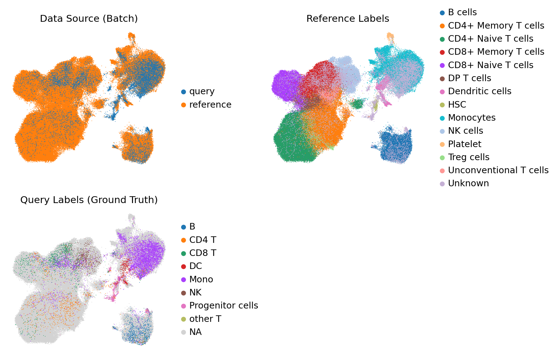
3.3 UMAP Visualization#
Visualize the shared space to verify that the Query data integrates well with the Reference.
[14]:
# Compute neighbors and UMAP
sc.pp.neighbors(adata, use_rep='z_c_joint')
sc.tl.umap(adata)

# Plot
sc.pl.umap(
    adata,
    color=['role', 'reference', 'query'],
    wspace=0.4,
    ncols=2,
    frameon=False,
    size=3,
    title=['Data Source (Batch)', 'Reference Labels', 'Query Labels (Ground Truth)']
)
4. Label Transfer via KNN#
We use a K-Nearest Neighbors classifier trained on the Reference embeddings to predict labels for the Query embeddings. ### 4.1 Defining Parallel Processing Helpers Efficiently predict using multiple CPU cores.
[11]:
# Import necessary modules for KNN
from sklearn.neighbors import KNeighborsClassifier
from sklearn.metrics import confusion_matrix, f1_score # f1_score and roc_auc_score might be used for evaluation
from joblib import Parallel, delayed
import seaborn as sns # For heatmap visualization
# Helper functions for parallel KNN prediction
def predict_batch(X, knn_model):
    """Predicts labels for a batch of data using the KNN model."""
    return knn_model.predict(X)

def predict_prob_batch(X, knn_model):
    """Predicts probability estimates for a batch of data using the KNN model."""
    return knn_model.predict_proba(X)

def knn_predict_par(X, knn_model, num_cores):
    """Performs parallel prediction using KNN."""
    X_batches = np.array_split(X, num_cores)
    with Parallel(n_jobs=num_cores, backend="threading") as parallel:
        results = parallel(delayed(predict_batch)(X_batch, knn_model) for X_batch in X_batches)
    return np.concatenate(results)

def knn_predict_prob_par(X, knn_model, num_cores):
    """Performs parallel probability prediction using KNN."""
    X_batches = np.array_split(X, num_cores)
    with Parallel(n_jobs=num_cores, backend="threading") as parallel:
        results = parallel(delayed(predict_prob_batch)(X_batch, knn_model) for X_batch in X_batches)
    return np.concatenate(results)
4.2 Training KNN and Prediction#
[ ]:
# 1. Train KNN on Reference Data
# Note: We use the whole embedding space, but valid labels are primarily from Reference
labels_with_unknown = adata.obs['reference']
knn = KNeighborsClassifier(n_neighbors=200, weights='uniform') # Adjust if need
knn.fit(adata.obsm['z_c_joint'], labels_with_unknown)

# 2. Predict on Query Data
query_mask = adata.obs['role'] == 'query'
X_query = adata[query_mask].obsm['z_c_joint']

# Use available cores (max 16 to avoid overhead)
num_cores = min(16, os.cpu_count())
prob_pred = knn_predict_prob_par(X_query, knn, num_cores)

# Optional: Inspect uncertainty
# prob_pred_unknown = prob_pred[:, np.where(knn.classes_ == 'Unknown')[0][0]]
# print(f"Average uncertainty: {np.mean(prob_pred_unknown):.4f}")

# 3. Determine Predicted Labels (Argmax)
predicted_indices = np.argmax(prob_pred, axis=1)
predicted_labels = knn.classes_[predicted_indices]

# Store results in AnnData
adata.obs['transfer'] = np.nan
adata.obs.loc[query_mask, 'transfer'] = predicted_labels
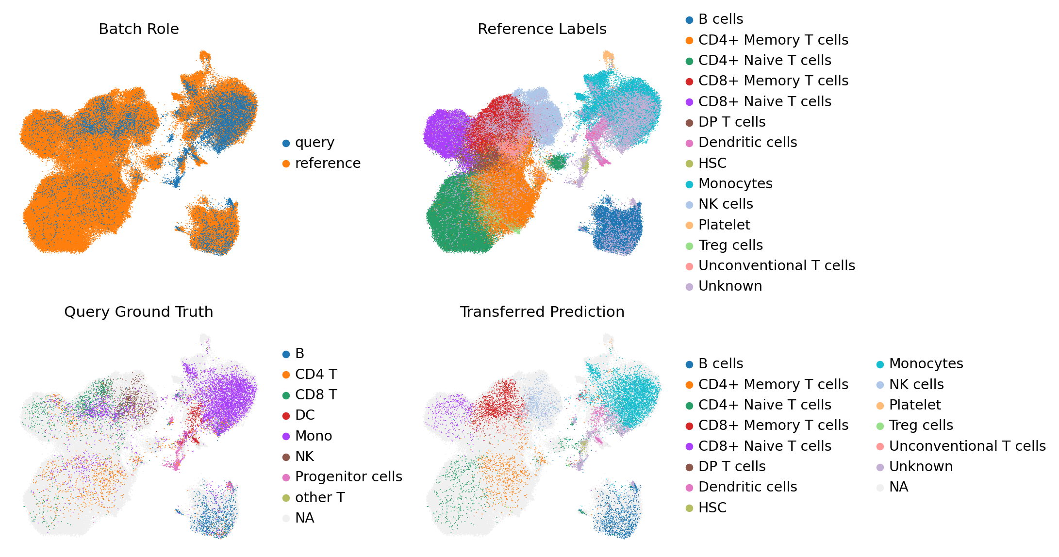
4.3 Visualization of Transferred Labels#
Compare the Ground Truth query labels with the Transferred labels.
[15]:
sc.pl.umap(
    adata,
    color=['role', 'reference', 'query', 'transfer'],
    na_color='#F0F0F0',
    size=3,
    frameon=False,
    wspace=0.4,
    ncols=2,
    title=['Batch Role', 'Reference Labels', 'Query Ground Truth', 'Transferred Prediction']
)
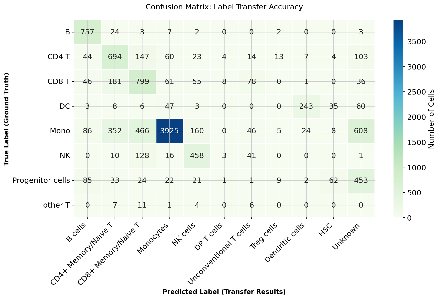
4.4 Evaluation: Confusion Matrix#
We calculate the confusion matrix to quantify the accuracy of the label transfer.
[16]:
# 1. Prepare Data
# Get all unique labels to ensure matrix dimensions match
all_kinds = np.unique(np.concatenate([label_query, predicted_labels]))
conf_matrix = confusion_matrix(label_query, predicted_labels, labels=all_kinds)
conf_matrix_df = pd.DataFrame(conf_matrix, index=all_kinds, columns=all_kinds)

# Filter to show only labels present in the Query dataset
present_labels = np.unique(label_query)
present_preds = np.unique(predicted_labels)
conf_matrix_df = conf_matrix_df.loc[present_labels, present_preds]

# 2. Group Subtypes for Cleaner Visualization
# Helper to merge columns
def merge_cols(df, new_col, cols_to_merge):
    valid_cols = [c for c in cols_to_merge if c in df.columns]
    if valid_cols:
        df[new_col] = df[valid_cols].sum(axis=1)
        df.drop(valid_cols, axis=1, inplace=True)
    return df

conf_matrix_df = merge_cols(conf_matrix_df, 'CD4+ Memory/Naive T', ['CD4+ Memory T cells', 'CD4+ Naive T cells'])
conf_matrix_df = merge_cols(conf_matrix_df, 'CD8+ Memory/Naive T', ['CD8+ Memory T cells', 'CD8+ Naive T cells'])

# 3. Reorder Columns for Logic
desired_order = [
    "B cells", "CD4+ Memory/Naive T", "CD8+ Memory/Naive T",
    "Monocytes", "NK cells", "DP T cells", "Unconventional T cells",
    "Treg cells", "Dendritic cells", "HSC", "Unknown"
]
plot_cols = [c for c in desired_order if c in conf_matrix_df.columns]
conf_matrix_df = conf_matrix_df[plot_cols]

# 4. Plot Heatmap
plt.figure(figsize=(12, 8))
ax = sns.heatmap(
    conf_matrix_df,
    linewidths=0.5,
    cmap="GnBu",
    annot=True,
    fmt='g',
    cbar_kws={'label': 'Number of Cells'}
)

# Improved Titles and Labels
ax.set_xlabel('Predicted Label (Transfer Results)', fontsize=12, fontweight='bold')
ax.set_ylabel('True Label (Ground Truth)', fontsize=12, fontweight='bold')
ax.set_title('Confusion Matrix: Label Transfer Accuracy', fontsize=14, pad=20)

plt.xticks(rotation=45, ha='right')
plt.yticks(rotation=0)
plt.tight_layout()
plt.show()
[ ]: